Demo looking at relationship between residuals and solar wind
Contents
Demo looking at relationship between residuals and solar wind#
Prep access to packages and dataset#
import os
import datetime as dt
import pooch
import pandas as pd
import numpy as np
import xarray as xr
import dask as da
from dask.diagnostics import ProgressBar
import zarr
# import holoviews as hv
# import hvplot.xarray
import matplotlib.pyplot as plt
from tqdm.auto import tqdm

from chaosmagpy.plot_utils import nio_colormap

from src.env import ICOS_FILE

TMPDIR = os.getcwd()
zarr_store = os.path.join(TMPDIR, "datacube_test.zarr")
print("Using:", zarr_store)

xr.set_options(
    display_expand_attrs=False,
    display_expand_data_vars=True
);
Using: /home/ash/code/geomagnetic_datacubes_dev/notebooks/datacube_test.zarr
zarr_store = os.path.join(TMPDIR, "datacube_test.zarr")
ds = xr.open_dataset(
    zarr_store, engine="zarr",
    chunks="auto"
)
Load information about the grid points#
The grid coordinates are stored in a separate file. These are locations within a spherical (theta, phi) shell. The grid_index matches up with the numbers given in the gridpoint_geo and gridpoint_qdmlt variables, so can be used to identify the (theta, phi) coordinates for each bin.
For
gridpoint_geo, (theta,phi) correspond to (90-Latitude,Longitude%360)For
gridpoint_qdmlt, (theta,phi) correspond to (90-QDLat,MLT*15)
# Load the coordinates, stored as "40962" within the HDF file.
gridcoords = pd.read_hdf(ICOS_FILE, key="40962")
# # Transform into a DataArray
# gridcoords = xr.DataArray(
#     data=gridcoords.values,
#     dims=("grid_index", "theta_phi"),
#     coords={
#         "grid_index": gridcoords.index,
#         "theta_phi": ["theta", "phi"]
#     }
# )
gridcoords["Latitude"] = 90 - gridcoords["theta"]
gridcoords["Longitude"] = np.vectorize(lambda x: x if x <= 180 else x - 360)(gridcoords["phi"])
gridcoords["QDLat"] = 90 - gridcoords["theta"]
gridcoords["MLT"] = gridcoords["phi"]/15
gridcoords
| theta | phi | Latitude | Longitude | QDLat | MLT | |
|---|---|---|---|---|---|---|
| 0 | 92.910599 | 125.730300 | -2.910599 | 125.730300 | -2.910599 | 8.382020 |
| 1 | 94.071637 | 127.340074 | -4.071637 | 127.340074 | -4.071637 | 8.489338 |
| 2 | 92.908770 | 127.341071 | -2.908770 | 127.341071 | -2.908770 | 8.489405 |
| 3 | 94.438861 | 126.233661 | -4.438861 | 126.233661 | -4.438861 | 8.415577 |
| 4 | 93.857171 | 125.428187 | -3.857171 | 125.428187 | -3.857171 | 8.361879 |
| ... | ... | ... | ... | ... | ... | ... |
| 40957 | 148.282526 | 90.000000 | -58.282526 | 90.000000 | -58.282526 | 6.000000 |
| 40958 | 121.717474 | 0.000000 | -31.717474 | 0.000000 | -31.717474 | 0.000000 |
| 40959 | 58.282526 | 0.000000 | 31.717474 | 0.000000 | 31.717474 | 0.000000 |
| 40960 | 121.717474 | 180.000000 | -31.717474 | 180.000000 | -31.717474 | 12.000000 |
| 40961 | 58.282526 | 180.000000 | 31.717474 | 180.000000 | 31.717474 | 12.000000 |
40962 rows × 6 columns
Reduce down to what we might actually work with#
ds points to the original dataset. In some cases we will just use _ds (defined below) which points to a subset of the data.
We will only consider the variable B_NEC_res_CHAOS-full which is the residual to the full CHAOS model (which parameterises the core, crustal, and magnetospheric fields), i.e. approximately the magnetic disturbance created by the ionosphere.
# Select out some interesting parameters to work with
_ds = ds[
    [
        "B_NEC_res_CHAOS-full",
        "Latitude", "Longitude", "QDLat", "QDLon", "MLT",
        # "SunZenithAngle", "OrbitNumber",
        "gridpoint_geo", "gridpoint_qdmlt",
        "IMF_BY", "IMF_BZ", "IMF_Em", "IMF_V",
        # "Kp", "RC", "dRC"
    ]
]
# Downsampled by 1/60 (i.e. 10-minute sampling) to make it easier to work on prototyping
_ds = _ds.isel(Timestamp=slice(0, -1, 60))
_ds
<xarray.Dataset>
Dimensions:               (Timestamp: 257807, NEC: 3)
Coordinates:
  * NEC                   (NEC) object 'N' 'E' 'C'
  * Timestamp             (Timestamp) datetime64[ns] 2014-05-01 ... 2019-04-3...
Data variables:
    B_NEC_res_CHAOS-full  (Timestamp, NEC) float64 dask.array<chunksize=(91667, 3), meta=np.ndarray>
    Latitude              (Timestamp) float64 dask.array<chunksize=(257807,), meta=np.ndarray>
    Longitude             (Timestamp) float64 dask.array<chunksize=(257807,), meta=np.ndarray>
    QDLat                 (Timestamp) float64 dask.array<chunksize=(257807,), meta=np.ndarray>
    QDLon                 (Timestamp) float64 dask.array<chunksize=(257807,), meta=np.ndarray>
    MLT                   (Timestamp) float64 dask.array<chunksize=(257807,), meta=np.ndarray>
    gridpoint_geo         (Timestamp) int64 dask.array<chunksize=(257807,), meta=np.ndarray>
    gridpoint_qdmlt       (Timestamp) int64 dask.array<chunksize=(257807,), meta=np.ndarray>
    IMF_BY                (Timestamp) float64 dask.array<chunksize=(257807,), meta=np.ndarray>
    IMF_BZ                (Timestamp) float64 dask.array<chunksize=(257807,), meta=np.ndarray>
    IMF_Em                (Timestamp) float64 dask.array<chunksize=(257807,), meta=np.ndarray>
    IMF_V                 (Timestamp) float64 dask.array<chunksize=(257807,), meta=np.ndarray>
Attributes: (2)Since we loaded the zarr using Dask, the dataset is not actually in memory. That will be useful later for scaling to the full dataset, but for now let’s load it into memory (so we can forget about Dask for now).
_ds.load()
<xarray.Dataset>
Dimensions:               (Timestamp: 257807, NEC: 3)
Coordinates:
  * NEC                   (NEC) object 'N' 'E' 'C'
  * Timestamp             (Timestamp) datetime64[ns] 2014-05-01 ... 2019-04-3...
Data variables:
    B_NEC_res_CHAOS-full  (Timestamp, NEC) float64 -9.226 -2.571 ... 0.3528
    Latitude              (Timestamp) float64 8.566 -29.69 ... -49.74 -11.29
    Longitude             (Timestamp) float64 -174.7 -175.3 -172.9 ... 63.8 63.9
    QDLat                 (Timestamp) float64 6.269 -33.49 ... -57.65 -19.68
    QDLon                 (Timestamp) float64 -103.4 -95.71 ... 118.0 135.2
    MLT                   (Timestamp) float64 12.46 13.14 15.61 ... 2.929 4.244
    gridpoint_geo         (Timestamp) int64 19702 12894 29903 ... 10071 31762
    gridpoint_qdmlt       (Timestamp) int64 19689 33951 28888 ... 40786 9717
    IMF_BY                (Timestamp) float64 nan 7.135 ... -0.7425 -0.9943
    IMF_BZ                (Timestamp) float64 nan -5.606 -4.719 ... 1.106 1.083
    IMF_Em                (Timestamp) float64 nan nan nan ... 0.03124 0.0314
    IMF_V                 (Timestamp) float64 nan 321.1 316.5 ... 310.7 nan
Attributes: (2)Some notes on those parameters:
The
IMF_..variables are created from OMNI data which has already been time-shifted to Earth’s bow shock, but also time-averaged over 20 minutes to give a smoothed input of energy to the magnetosphere and account for typical lag times from the input at the magnetopause to the response in the ionosphere. This should be pretty much the same input as that used in the AMPS model. For a better model we should use the full original OMNI data as input (both to give the full time-history to drive the model better, but also open up the opportunity for the model to account for varying lag times - we expect a more prompt response on the dayside, “direct driving”, and a much more variable lagged response on the nightside, “magnetospheric unloading”).IMF_Emis merging electric field (a type of coupling function, composed fromBY,BZ&V)gridpoint_geoandgridpoint_qdmltare indexes into positions in spherical grids of 40962 points. Use thegridcoordsdataframe to identify coordinates of those points
Some inspection of the data#
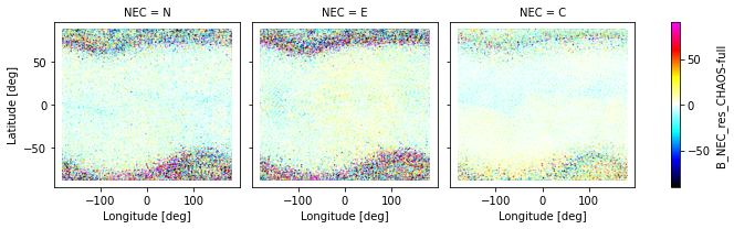
_ds.plot.scatter(
    x="Longitude", y="Latitude", hue="B_NEC_res_CHAOS-full",
    s=0.1, cmap=nio_colormap(), col="NEC", robust=True
)
<xarray.plot.facetgrid.FacetGrid at 0x7f82e16b5fa0>
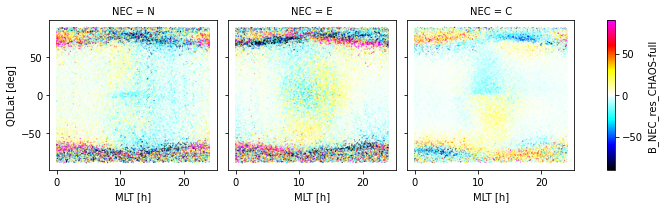
_ds.plot.scatter(
    x="MLT", y="QDLat", hue="B_NEC_res_CHAOS-full",
    s=0.1, cmap=nio_colormap(), col="NEC", robust=True
)
<xarray.plot.facetgrid.FacetGrid at 0x7f82d8720fa0>
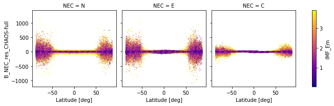
_ds.plot.scatter(
    x="Latitude", y="B_NEC_res_CHAOS-full", hue="IMF_Em",
    s=0.1, cmap="plasma", col="NEC", robust=True
)
<xarray.plot.facetgrid.FacetGrid at 0x7f82d864dac0>
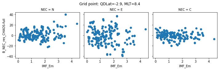
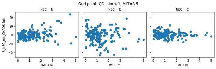
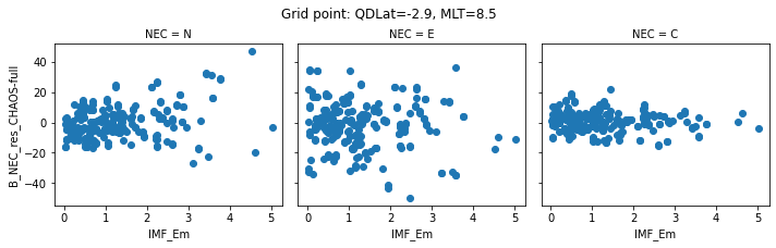
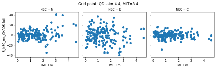
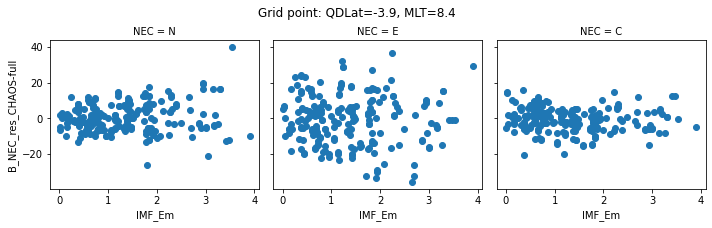
def inspect_gridpoint(_ds=_ds, index=0, x="IMF_Em"):
    """Quick scatterplot of data in a given bin"""
    # Select data from given gridpoint
    __ds = _ds.where(ds["gridpoint_qdmlt"]==index, drop=True)
    # Identify coordinates of that bin
    qdlat, mlt = gridcoords.iloc[index][["QDLat", "MLT"]]
    # Construct figure
    facetgrid = __ds.plot.scatter(x=x, y="B_NEC_res_CHAOS-full", col="NEC")
    # Add coordinates for the displayed gridpoint
    facetgrid.fig.suptitle(
        f"Grid point: QDLat={np.round(qdlat, 1)}, MLT={np.round(mlt, 1)}",
        verticalalignment="bottom"
    )
    return facetgrid


# Plot a few different bins. NB: We use the full dataset this time
for index in range(0, 5):
    inspect_gridpoint(_ds=ds, index=index)
A simple model based on linear regressions within each bin#
Within each bin, we perform a linear regression of B_NEC_res_CHAOS-full against IMF_Em.
Using the full dataset ds this time - but we chop it in half - using the first half for training and the second half for testing
We ignore the radial variation of data within each bin. This is okay because data are collected at a similar altitude since we only consider one satellite over five years. We will need to re-think this when extending to longer duration and multiple satellites.
Use only the vertical component, just to keep things simpler. The vertical component is the more stable one so easier to predict (maybe?).
Divide the dataset in two: (use the first half to train the model, and the second half to test it)
midpoint = int(len(ds["Timestamp"])/2)
_ds_train = ds.isel(Timestamp=slice(0, midpoint, 1))  # used to build the model
_ds_test = ds.isel(Timestamp=slice(midpoint, -1, 1))  # used to test the model
_ds_train["Timestamp"].data
array(['2014-05-01T00:00:00.000000000', '2014-05-01T00:00:10.000000000',
       '2014-05-01T00:00:20.000000000', ...,
       '2016-10-28T04:45:40.000000000', '2016-10-28T04:45:50.000000000',
       '2016-10-28T04:46:00.000000000'], dtype='datetime64[ns]')
_ds_test["Timestamp"].data
array(['2016-10-28T04:46:10.000000000', '2016-10-28T04:46:20.000000000',
       '2016-10-28T04:46:30.000000000', ...,
       '2019-04-30T23:59:20.000000000', '2019-04-30T23:59:30.000000000',
       '2019-04-30T23:59:40.000000000'], dtype='datetime64[ns]')
from scipy.stats import linregress
First attempt using groupby-apply workflow didn’t work out…
# def regress_xarray(ds, x="IMF_Em", y="B_NEC_res_CHAOS-full"):
#     """Regress variables within a dataset against each other

#     Returns a DataArray so that it can be used in a groupby-apply workflow...
#     Construction of this must be really slow - need to investigate how to do this properly
#     """
#     regression = linregress(ds[x], ds[y])
#     # return [regression.slope, regression.intercept]
#     return xr.DataArray(
#         data=[regression.slope, regression.intercept],
#         dims=["slope_intercept"], coords={"slope_intercept": ["slope", "intercept"]}
#     )

# %%time
# regression_results = _ds_train.sel(NEC="C").groupby("gridpoint_qdmlt").apply(regress_xarray)
def build_model(ds=_ds_train):
    """Returns a DataArray containing slopes & intercepts of each linear regression"""
    x = "IMF_Em"
    y = "B_NEC_res_CHAOS-full"
    N = len(ds["Timestamp"])
    # chunksize = 100000
    # ds = ds.chunk(chunksize)
    # Arrange the x-y data to be regressed
    # Read the data from the input Dataset (ds) and put in a simpler DataArray
    regression = xr.DataArray(
        data=np.empty((N, 2)),
        dims=["Timestamp", "dim_1"],
        coords={
            "gridpoint_qdmlt": ds["gridpoint_qdmlt"]
        }
    )#.chunk(chunksize)
    regression.data[:, 0] = ds[x].data
    regression.data[:, 1] = ds[y].sel(NEC="C").data
    # Load it into memory - not doing so makes it very slow
    regression.load()
    # Remove entries with NaNs so that lingress works
    regression = regression.where(~np.any(np.isnan(regression), axis=1), drop=True)

    def _regress(da):
        result = linregress(da.data[:, 0], da.data[:, 1])
        return [result.slope, result.intercept]

    regression_results = np.empty((40962, 2))
    regression_results[:] = np.nan
    # Split dataset into the bins and apply the regression within each bin.
    for i, __da in tqdm(regression.groupby("gridpoint_qdmlt")):
        regression_results[int(i)] = _regress(__da)

    regression_results = xr.DataArray(
        data=regression_results,
        dims=["gridpoint_qdmlt", "slope_intercept"],
        coords={
            "gridpoint_qdmlt": range(40962),
            "slope_intercept": ["slope", "intercept"]
        }
    )
    return regression_results
regression_results = build_model(ds=_ds_train)
regression_results
<xarray.DataArray (gridpoint_qdmlt: 40962, slope_intercept: 2)>
array([[ -0.91064602,   0.92471419],
       [ -0.35233481,   2.36205458],
       [ -1.08103889,   2.55874955],
       ...,
       [  0.76851364,  -0.45965504],
       [ -0.21283606,  11.07832005],
       [ -0.45352056, -12.87865929]])
Coordinates:
  * gridpoint_qdmlt  (gridpoint_qdmlt) int64 0 1 2 3 ... 40958 40959 40960 40961
* slope_intercept (slope_intercept) <U9 'slope' 'intercept'Apply the regression results to make the predictions over the test dataset#
def make_predictions(ds, regression_results):
    """Returns a DataArray of predictions for B_NEC_res based on IMF_Em"""
    # Create a DataArray to hold the predictions
    prediction = xr.DataArray(
        data=np.empty((len(ds["Timestamp"]), 2)),
        coords={
            "gridpoint_qdmlt": ds["gridpoint_qdmlt"].data,
            "slope_intercept": ["slope", "intercept"],
        },
        dims=("gridpoint_qdmlt", "slope_intercept")
    )
    # Reorganise the regression results to follow the order of the gridpoints in the dataset
    prediction.data = regression_results.reindex_like(prediction).data
    # Apply the regression results, inplace in the prediction DataArray
    m = prediction.sel({"slope_intercept": "slope"}).data
    c = prediction.sel({"slope_intercept": "intercept"}).data
    prediction.data[:, 0] = m * ds["IMF_Em"].data + c
    # Drop the unneeded dimension
    prediction = prediction.isel({"slope_intercept": 0}).drop("slope_intercept")
    # Set Timestamp as the coordinate
    prediction = prediction.rename({"gridpoint_qdmlt": "Timestamp"})
    prediction["Timestamp"] = ds["Timestamp"]
    return prediction
prediction = make_predictions(_ds_test, regression_results)
# # Remove some of the unreasonably large predictions
# prediction = prediction.where(~(np.fabs(prediction) > 1000))
# prediction
prediction
<xarray.DataArray (Timestamp: 7734201)>
array([ 8.95574744, 10.24684501, 10.36732238, ...,  0.97471219,
        1.33689136,  1.09296473])
Coordinates: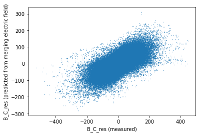
* Timestamp (Timestamp) datetime64[ns] 2016-10-28T04:46:10 ... 2019-04-30T...fig, ax = plt.subplots(1, 1)
ax.scatter(_ds_test["B_NEC_res_CHAOS-full"].sel(NEC="C").data, prediction.data, s=0.1)
ax.set_xlabel("B_C_res (measured)")
ax.set_ylabel("B_C_res (predicted from merging electric field)");
_ds_test["prediction"] = prediction
_ds_test["prediction_residual"] = prediction - \
_ds_test["B_NEC_res_CHAOS-full"].sel(NEC="C")
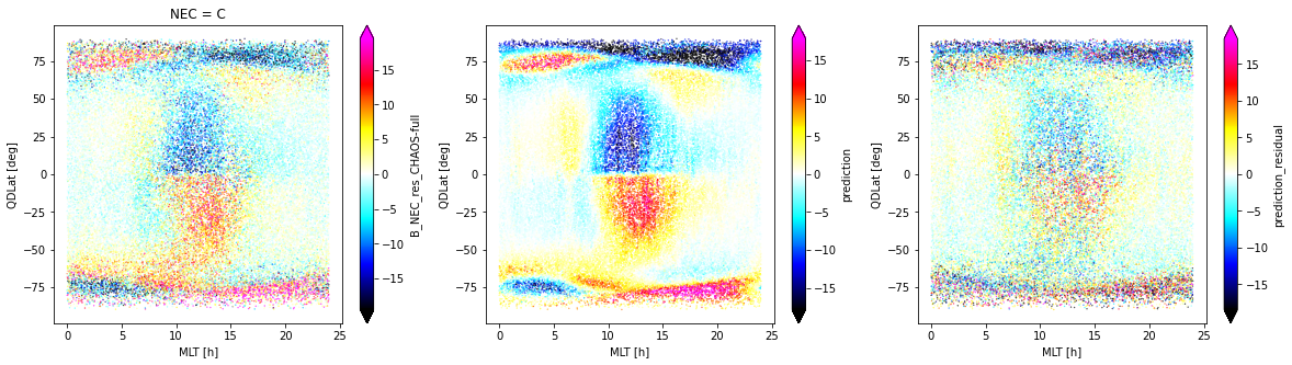
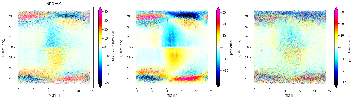
fig, axes = plt.subplots(nrows=1, ncols=3, figsize=(20, 5))
_ds_test.isel(Timestamp=slice(0, -1, 60)).sel(NEC="C").plot.scatter(
x="MLT", y="QDLat", hue="B_NEC_res_CHAOS-full",
s=0.1, cmap=nio_colormap(), robust=True, ax=axes[0]
)
_ds_test.isel(Timestamp=slice(0, -1, 60)).plot.scatter(
x="MLT", y="QDLat", hue="prediction",
s=0.1, cmap=nio_colormap(), robust=True, ax=axes[1]
)
_ds_test.isel(Timestamp=slice(0, -1, 60)).plot.scatter(
x="MLT", y="QDLat", hue="prediction_residual",
s=0.1, cmap=nio_colormap(), robust=True, ax=axes[2]
)
<matplotlib.collections.PathCollection at 0x7f82e11b27f0>
Repeat the above with only quiet data#
quiet = (ds["Kp"] < 3) & (ds["IMF_Em"] < 0.8)
ds_quiet = ds.where(quiet)

midpoint = int(len(ds["Timestamp"])/2)
_ds_train_quiet = ds_quiet.isel(Timestamp=slice(0, midpoint, 1))
_ds_test_quiet = ds_quiet.isel(Timestamp=slice(midpoint, -1, 1))
# t_0 = ds["Timestamp"].isel(Timestamp=0)
# t_mid = ds["Timestamp"].isel(Timestamp=int(len(ds["Timestamp"])/2))
# t_mid
# _ds_train_quiet.isel(Timestamp=slice(0, -1, 60)).plot.scatter(
#     x="MLT", y="QDLat", hue="B_NEC_res_CHAOS-full",
#     s=0.1, cmap=nio_colormap(), col="NEC", robust=True
# )
regression_results_quiet = build_model(ds=_ds_train_quiet)
prediction_quiet = make_predictions(_ds_test_quiet, regression_results_quiet)
prediction_quiet
<xarray.DataArray (Timestamp: 7734201)>
array([       nan,        nan,        nan, ..., 1.05331635, 1.80006575,
       1.99285837])
Coordinates: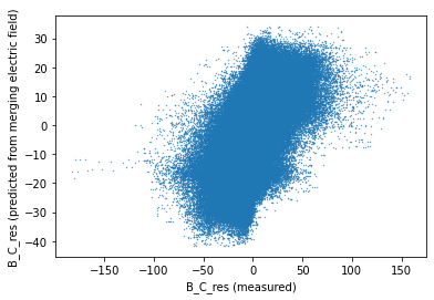
* Timestamp (Timestamp) datetime64[ns] 2016-10-28T04:46:10 ... 2019-04-30T...fig, ax = plt.subplots(1, 1)
ax.scatter(_ds_test_quiet["B_NEC_res_CHAOS-full"].sel(NEC="C").data, prediction_quiet.data, s=0.1)
ax.set_xlabel("B_C_res (measured)")
ax.set_ylabel("B_C_res (predicted from merging electric field)");
_ds_test_quiet["prediction"] = prediction_quiet
_ds_test_quiet["prediction_residual"] = prediction_quiet - \
    _ds_test_quiet["B_NEC_res_CHAOS-full"].sel(NEC="C")

fig, axes = plt.subplots(nrows=1, ncols=3, figsize=(20, 5))
_ds_test_quiet.isel(Timestamp=slice(0, -1, 60)).sel(NEC="C").plot.scatter(
    x="MLT", y="QDLat", hue="B_NEC_res_CHAOS-full",
    s=0.1, cmap=nio_colormap(), robust=True, ax=axes[0]
)
_ds_test_quiet.isel(Timestamp=slice(0, -1, 60)).plot.scatter(
    x="MLT", y="QDLat", hue="prediction",
    s=0.1, cmap=nio_colormap(), robust=True, ax=axes[1]
)
_ds_test_quiet.isel(Timestamp=slice(0, -1, 60)).plot.scatter(
    x="MLT", y="QDLat", hue="prediction_residual",
    s=0.1, cmap=nio_colormap(), robust=True, ax=axes[2]
)
<matplotlib.collections.PathCollection at 0x7f828574d1f0>